Category Archives: PCA

Dense South Asian ChromoPainter

I had run ChromoPainter/fineSTRUCTURE for 715 South Asians using only about 90,000 SNPs. I thought it would be a useful exercise to use more SNPs, so I had to drop the Reich et al dataset. That left me with 615 individuals and 418,854 SNPs.

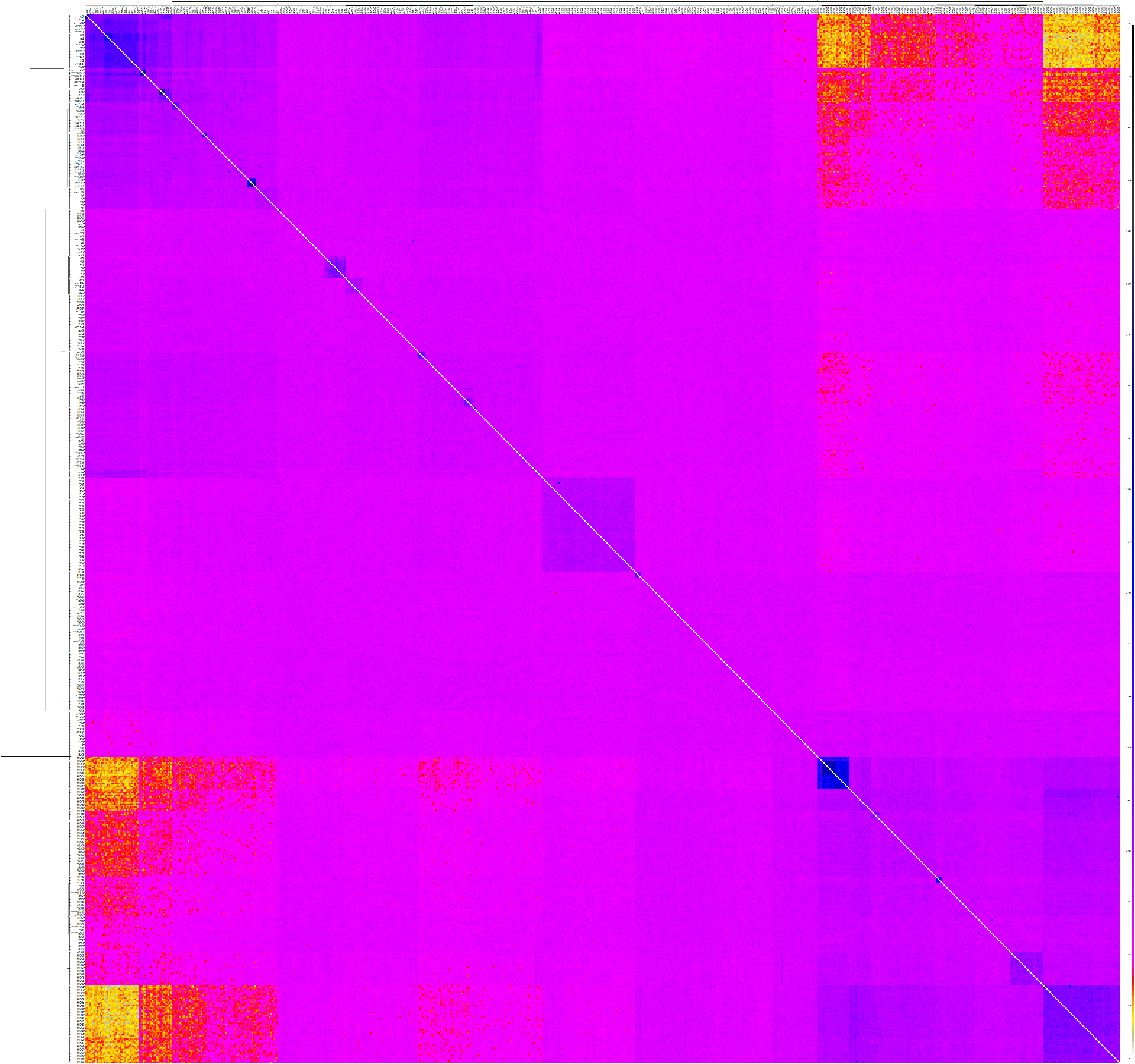
The "chunkcounts" file has the donors in columns and recipients in rows. Here's a heat map of the same.

fineSTRUCTURE classified these 615 individuals into 89 clusters. I have named these clusters for convenience, however, the names do not imply that anyone in the Punjab cluster is Punjabi.

While I created the cluster tree at the top of the spreadsheet, here's how the clusters are related.

The most interesting thing is how Gujarati A (likely Patels) are an out-group to everyone else. Another major grouping is that of the Baloch, Brahui and Makrani, along with 4 Sindhis (might be one of the Baloch tribe of Sindh?).

The Punjabis, Sindhis and Pathan get better classification here than they did last time.

The Punjab cluster includes 3 Gujarati B, 4 Pathans, 2 Singapore Indians, Punjabis, Haryanvis, Kashmiris, and a Rajasthani Brahmin. Even using this method, HRP0036, who is half-Sri Lankan and half-German/Polish was classified in the same cluster.

The Dharkar and Kanjar could not be separated at all here. According to Metspalu:

There are three second degree relatives groups in our sample: ..snip.. [Kanjar evo_37 and Dharkar HA023]. Again the last pair needs further explanation. The Dharkar and Kanjar practice a nomadic lifestyle and were living side by side at the time of sampling. As the ethnic border between the two is permeable we cannot rule out neither our error during sample collection and/or subsequent labelling nor shifted self-identity.

The inter-cluster heat map:

And you can see the chunkcounts donated from each cluster to recipient individuals in a spreadsheet.

The pairwise coincidence:

And the PCA plots:

ChromoPainter/fineStructure South Asians

You have probably heard of ChromoPainter/fineSTRUCTURE by now (Eurogenes, Dienekes, MDLP and Razib).

So I decided to run the South Asian samples data which I had earlier done PCA/MClust on through ChromoPainter and fineSTRUCTURE.

Here is the coancestry matrix among the 715 participants visualized as a heat map.

UPDATE: Here's a huge image showing the same.

fineSTRUCTURE can use this coancestry matrix to classify individuals into clusters, 52 in this case (compared to 38 using PCA and MClust). You can check the cluster assignments in a spreadsheet.

Note that I have named the clusters. That's just a shorthand so we don't have to refer to them by cluster number. Instead I used the population with the largest number of individuals in a cluster to label that cluster.

Here's the cluster-level coancestry heat map.

And the pairwise coincidence:

And finally PCA plots for the first 10 dimensions from fineSTRUCTURE.

UPDATE (Feb 9, 2012): New PCA plots with better markers for the clusters.

South Asian PCA 3D Plot

Here's a 3-D plot of my South Asian PCA run, showing the first three principal components.

The principal components have been scaled according to their respective eigenvalues. The plot is rotating about the vertical 1st eigenvector.

You can find out your position on the plot by using the dropdown below the plot and selecting your Harappa ID.

South Asian PCA Plots

I did a South Asian PCA + Mclust analysis last month. Here are the PCA plots from that analysis.

First, the eigenvectors are not scaled to the eigenvalues in the plots. So here's a table explaining how much each eigenvector is worth.

Eigenvector Percentage variation explained
1 1.134%
2 0.452%
3 0.351%
4 0.263%
5 0.254%
6 0.236%
7 0.228%
8 0.224%
9 0.215%
10 0.209%
11 0.207%
12 0.205%
13 0.203%
14 0.201%
15 0.198%
16 0.194%
17 0.191%
18 0.189%
19 0.189%
20 0.188%
21 0.188%
22 0.187%
23 0.186%
24 0.185%
25 0.184%
26 0.184%
27 0.183%
28 0.182%
29 0.180%
30 0.180%
31 0.179%
32 0.179%

Eigenvector 1 looks like the Indian cline but it's actually a West-East Eurasian cline. It's quite similar to Reich et al's Indian cline for their subset of populations (correlation between pc1 and ASI is 0.998869) but since East Asian is not separated out here due to the lack of any East Asian samples, we get a mix of East Asian and Ancestral South Indian towards the right of the plot.

Eigenvector 2 separates Kalash from everyone else.

South Asian PCA + Mclust

I combined reference 3 with Metspalu et al data and Harappa Ancestry Project participants (up to HRP0200). Then I kept only those individuals whose combined proportion of South Asian and Onge components on my reference 3 admixture results was more than 50%.

I ran PCA on these South Asian samples and kept 31 dimensions. Running Mclust on the PCA results gave me 37 clusters.

The clustering results are in a spreadsheet.

For an individual, the value under a specific cluster shows the probability of that person belonging to that cluster. For example, HRP0152 has a 58% probability of belonging to cluster CL8 and 42% probability of being in cluster CL14.

For the populations in the first sheet, I added up the probabilities of all the samples in that population to get the expected number of individuals of that ethnicity belonging to a specific cluster.

In the second sheet, I have listed all the individual samples' clustering results.

There are some outliers who didn't belong in any cluster: HRP0001 (me, of course), 7 (out of 18) Makranis, 4 (out of 23) Sindhis, 3 (all) Great Andamanese, 1 (out of 20) Balochi, 1 (out of 4) Madiga, and 1 (only) Onge.

Reference 3 + Yunusbayev + HAP PCA and Mclust

I ran Principal Component Analysis (PCA) on reference 3 along with Yunusbayev et al Caucasus dataset and Harappa Ancestry Project participants (up to HRP0200).

Then I ran mclust on the first 70 dimensions. The resulting 156 clusters can be seen in a spreadsheet.

For individuals belonging to Harappa Ancestry Project, the value in a column shows that person's probability of being in that cluster. So if there is a 1 in CL15 for example, then that person has a 100% probability of being in Cluster CL15.

For the reference population groups, I have added up the probabilities for all the individuals belonging to that group.

Reference 3 + HAP PCA

I had run PCA on the Reference 3 dataset before. Now I included Harappa participants in it as well.

Here's the dendrogram based on the Euclidean distance between Harappa participants in their PCA results.

Since no one liked the IBS nearest neighbors lists, I thought making a spreadsheet with every participants' closest 100 neighbors in PCA space might be more fruitful.

Note that for the Harappa participants, the median distance to their nearest neighbor is 0.2064. So if your nearest neighbor is more than let's say 0.3 away, then you are not close to anyone.

Indian Cline III

I have been working on creating 100% ASI (Ancestral South Indian) samples recently. So it was really interesting that Dienekes did similar experiments:

I am going about creating the "pure" allele frequencies somewhat differently, so that would be a useful exercise.

Anyway, I thought you guys would be itching for some new results. So here's a PCA plot:

This used the same Principal Component Analysis as the one here using the 96 Indian Cline samples, Utahn Whites and Onge. However, I projected three extra "populations" on this plot.

These three populations are simulated genetic data of 25 individuals using the allele frequencies from Reference 3 Admixture results.

  1. Onge11 is generated from the Onge (C2) component from K=11 admixture for Reference 3.
  2. SA11 is generated from the South Asian (C1) component from the same K=11 admixture.
  3. SA12 is generated from the South Asian (C1) component from the K=12 admixture.

As you can see, the SA12 population lies between 100% ASI and the Indian Cline samples.

The Onge11 generated samples are a bit beyond 100% ASI on the first principal component, but they are also shifted towards the real Onge on pc2.

Indian Cline II

One thing I forgot in the post yesterday about the Indian cline was to try to extrapolate from the PCA results to 100% ANI (Ancestral North Indian) and 100% ASI (Ancestral South Indian).

This is a simple linear extrapolation which should be okay since PCA is linear.Men's Club - Онлайн Журнал

The "N" denotes the extrapolated position of ANI and "S" denotes the ASI. The points to the left of "N" are all Utahn Whites while the Onge are on the bottom right of the graph.

As you can see, the ASI is about the same as Onge in terms of eigenvector 1 (which represents the Indian cline approximately), but ASI is far from Onge on the 2nd eigenvector. That is expected since the Onge have been separated from the mainland populations for a long time.

The more interesting thing is that the extrapolated position of ANI is a little to the right of all the Utahn Whites.

We'll need a similar analysis of the Indian cline with more populations to see which one the ANI is closest to.

PS. I should point out that I am using correlation between a limited number of population statistics to find a relationship between the 1st principal component and Reich et al's ASI estimate. This has a number of drawbacks. It would be much better to compute ASI directly.

Indian Cline

I had used linear regression to estimate Ancestral South Indian (ASI) component from Reference 3 K=11 admixture run. Now here are a couple more exercises along the same lines but much simpler.

Just using the 96 Indian cline samples from Reich et al to compute PCA or admixture doesn't work as the Chenchu separate out in both analyses from the rest. So I added the Utahn White (CEU) samples from HapMap and the Onge from Reich et al.

First, I ran supervised admixture with two ancestral components, Utahn Whites and Onge. Here's the Onge component plotted against Reich et al's ASI estimate along with a linear regression estimate. The correlation between the two is 0.9908.

Second, I ran Principal Component Analysis (PCA) on the Indian cline samples plus Utahn Whites and Onge. Here are the first two PCA dimensions plotted. The first eigenvector explains 4.04% of the total variation and the 2nd explains 1.94%.

The first principal component is mostly along the Indian cline while the second one basically separates the Onge from everyone else.

Using the 1st principal component to estimate ASI, here's the plot with Reich et al's ASI estimate along with a regression line. The correlation between pc1 and ASI is 0.9929.

Note that both these methods work only if the samples are on the Indian cline, i.e., they don't have any other admixture.

And now for comparison, here's the linear regression for the Reference 3 K=11 admixture Onge component and ASI. The correlation here is 0.9949. Note that this is a little different than my previous analysis since I calculated the population averages using only the 96 samples recommended by Reich et al.

Here's a spreadsheet containing the data for these three runs.

There are a couple more tricks I have to figure out some things regarding Ancestral South Indian admixture. Let's hope they provide us some insight.