Monthly Archives: March 2011 - Page 2

Reference I PCA

I ran PCA on the Reference I dataset which includes 2,654 samples from various populations.

Here are the top ten eigenvalues:

  • 178.727040
  • 118.884690
  • 15.014072
  • 9.346602
  • 5.983225
  • 5.140090
  • 3.322723
  • 2.739313
  • 2.559640
  • 2.475389

While the first two eigenvalues are much bigger than the rest, the first explains 6.82% of the variation and the second 4.54%, the Tracy-Widom stats show that about 70-something eeigenvectors are significant.

Here are the plots for the first 10 principal components. Remember that the 1st eigenvector is 1.5 times the 2nd.

Here is a 3-D PCA plot (hat tip: Doug McDonald) showing the first three eigenvectors. The plot is rotating about the 1st eigenvector which is vertical. Also, I have stretched the principal components based on the corresponding eigenvalues.

I also ran MClust on the PCA data and got 16 clusters. The results are in a spreadsheet. I am sure with more principal components than the 10 I used, I would be able to deduce finer population structure.

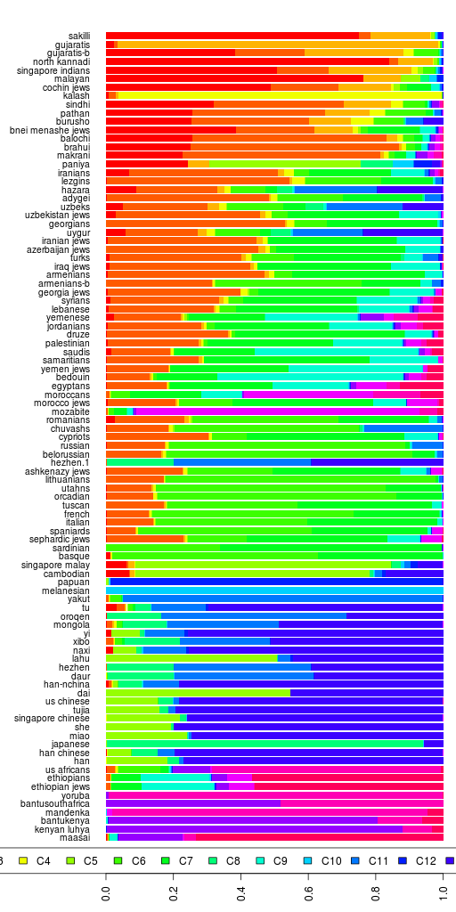
Note that African Americans cluster with East Africans in CL1. That's because African Americans have some European ancestry (20% on average) and that pulls them away from West Africans and towards Europeans. East Africans also lie in that direction, so they cluster together in a PCA. However, that doesn't mean that African Americans have East African ancestry. If you look at the Admixture results for African Americans, you see that their East African ancestry is negligible.

Iranians

Since we have 7 Iranians in the project, it's time to look at them as a group. We also have 19 Iranians from the Behar et al dataset.

Let's look at their admixture results at K=12.

The big difference between Harappa Project Iranians and Behar et al Iranians is African admixture. Only one Harappa Iranian (HRP0046) has 1% African admixture while three Behar Iranians have more than 10%.

Let's do hierarchical clustering with complete linkage using the Euclidean distance between admixture components. First a caveat or two. This is not a phylogeny. Also, the Euclidean distance measure is not a good one for measuring differences in admixture but I am not sure what would be better.

HRP0010 who is an Assyrian actually clusters better with Caucasian, Iranian and Iraqi Jews than with Iranians.

I'll run an MDS or PCA of the whole region from Punjab/Kashmir to the Levant and Caucasus soon which should be more interesting for clustering.

UPDATE: Since Palisto wondered, I checked and found out that he, an Iraqi Kurd, is very like the Iranians in his admixture result. So I have included him (HRP0059).

Admixture: Choice of K

Admixture lets you choose the number of ancestral populations, K. This number is really important and in a lot of cases we do not know how many ancestral populations our samples have descended from. In the Admixture manual, we are advised:

Use ADMIXTURE's cross-validation procedure. A good value of K will exhibit a low cross-validation error compared to other K values. Cross-validation is enabled by simply adding the --cv flag to the ADMIXTURE command line. In this default setting, the cross-validation procedure will do 10 repetitions, each time holding out 10% of the genotypes at
random.

I like this idea compared to using the BIC (Bayes Information Criterion) but I am plotting all the different variables for various K below.

For our Reference I dataset which is what I have used for most of the analysis so far, here is the spreadsheet for Log Likelihood, BIC, AIC and CV (cross-validation error). The plots follow.

Using the cross-validation error, the optimum value of K so far is 17 which is the largest I have run so far. It now takes days to run admixture (with cross-validation). Cross-validation almost doubles the time required to run.

For Reference II, here are the spreadsheet and graphs.


The cross-validation error is lowest at K=16 which is the highest I have run. So it is likely to decrease further for higher K.

Ref1 South Asian + Harappa MDS MClust

Now I am going nuts on this dataset consisting of South Asians (minus Kalash and Hazara) from Reference I and some Harappa participants, but I promise this is the last item on this specific data. I will however do similar analyses some time after integrating all the new South Asian samples I have gotten (via project participation as well as from research data).

I ran MDS on the data in Plink and then retaining various number of MDS dimensions, ran MClust on it. This is what Dienekes calls Clusters Galore.

Here are the plots of the MDS, two dimensions at a time.

The graph of number of MDS dimensions retained versus optimum number of clusters computed by Mclust is as follows:

The maximum number of clusters (28) are inferred with 8 MDS dimensions. So I posted the clustering results for 8 MDS dimensions + 28 clusters.

Some observations on the clusters:

  1. 56 of the 62 Gujaratis are in cluster CL1 and the remaining 6 are in CL5. Both are Gujarati-only clusters. Let's see where the Harappa Gujaratis fall next time I do this analysis,
  2. CL2 has an Andhra Reddy, Caribbean Indians, a Keralan, a few Gujaratis-B, and a third of the Singapore Indians.
  3. Gujaratis-B are a varied lot spread out into CL3, CL7, CL2, CL8, CL4, CL6, and CL15, but half are in CL3.
  4. CL6 has a lot of the South Indian Brahmins
  5. Burusho are isolated
  6. Punjabis from the project seem to be divided among CL7, CL8 and CL15.

I also posted the results for 20 MDS dimensions resulting in 21 clusters.

Ref1 South Asians + Harappa PCA Clusters II

Using the PCA data for Reference I South Asians plus project participants, Sriram computed a tree-based clustering called clique optimization. The result for that is a pdf file. Take a look!

Thanks, Sriram!Балки

Ref1 South Asian + Harappa Admixture

Since I was working on this dataset consisting of South Asians (minus Kalash and Hazara) from Reference I and some Harappa participants, I thought I would run Admixture on it.

The optimum value for the number of ancestral populations K is 3 in this case. Roughly the three ancestral components correspond to South India, Balochistan and Gujarat.

The spreadsheet showing the admixture results is here. The first sheet shows the individual results for reference samples as well as project participants.

The 2nd sheet shows the average (and standard deviation) for the reference populations.

The 3rd sheet shows the average and standard deviation for each cluster computed by MClust. I included only the samples which had at least 90% probability of belonging to a cluster.

Note how clusters CL8, CL9 and CL13 have a lot more variation than the others. Of course, I am in CL9 along with some fairly eclectic samples.

Reference I Admixture Analysis K=17

Continuing with Reference I admixture analysis, here is the results spreadsheet.

You can click on the legend to the right of the bar chart to sort by different ancestral components.

If you can't see the interactive chart above, here's a static image.

C1 South Asian C2 Balochistan/Caucasus
C3 Gujarati C4 Kalash
C5 Southeast Asian C6 European
C7 Mediterranean C8 Japanese
C9 Southwest Asian C10 Melanesian
C11 Siberian C12 Papuan
C13 Chinese C14 Eastern Bantu
C15 Northwest African C16 West African
C17 East African

The new ancestral component is the tightly clustered Gujarati. This consists of almost two-thirds of the Gujaratis sampled by HapMap in Houston, TX. So my question is does anyone have any idea which Gujarati communities are the biggest in Houston? I know that Patel is a very common name, probably the most common South Asian last name in the US. Most Patels I know have been from Gujarat. Are Patels a tightly knit community who are endogamous but likely don't marry close cousins? Are there different Patel subcommunities?

Fst divergences between estimated populations for K=17:

Here are the Fst numbers:

C1 C2 C3 C4 C5 C6 C7 C8 C9 C10 C11 C12
C2 0.072
C3 0.032 0.044
C4 0.076 0.061 0.062
C5 0.085 0.120 0.085 0.129
C6 0.076 0.045 0.059 0.072 0.123
C7 0.085 0.062 0.073 0.088 0.138 0.050
C8 0.084 0.119 0.084 0.128 0.035 0.122 0.138
C9 0.091 0.059 0.076 0.095 0.139 0.062 0.058 0.139
C10 0.168 0.203 0.168 0.215 0.171 0.206 0.220 0.172 0.221
C11 0.090 0.116 0.088 0.127 0.064 0.117 0.135 0.039 0.138 0.188
C12 0.188 0.225 0.189 0.237 0.209 0.228 0.242 0.207 0.243 0.145 0.220
C13 0.086 0.122 0.087 0.130 0.030 0.125 0.140 0.014 0.142 0.173 0.044 0.210
C14 0.151 0.155 0.146 0.177 0.186 0.163 0.164 0.186 0.152 0.257 0.190 0.275
C15 0.089 0.066 0.076 0.096 0.133 0.060 0.054 0.132 0.063 0.211 0.131 0.232
C16 0.160 0.164 0.155 0.186 0.194 0.173 0.173 0.195 0.162 0.265 0.199 0.283
C17 0.114 0.111 0.107 0.136 0.150 0.119 0.114 0.151 0.106 0.223 0.154 0.242
C13 C14 C15 C16
C14 0.188
C15 0.135 0.115
C16 0.197 0.013 0.122
C17 0.153 0.034 0.079 0.041

PS. This was run using Admixture version 1.04 so I can make an apples-to-apples comparison with the previous runs.

Dienekes on ANI/ASI

Dienekes has a word of caution about choosing reference populations and admixture results.

Consider a sample of 25 Mexicans from the HapMap and 25 Yoruba from the Hapmap, 25 Iberian Spanish from the 1000 Genomes Project, and 25 Pima from the HGDP as parental populations. We obtain for our Mexican sample:

  • 59.7% European
  • 36.9% "Native American"
  • 3.4% African

Let's run a final experiment with just the Mexicans, Spanish, and Yoruba, i.e., with no Native American samples. At K=3 we obtain:

  • 70% "Native American"
  • 29.7% European
  • 0.4% African

The "Native American" component has increased again! The explanation is simple: as we exclude less admixed Native American groups, Mexicans appear (comparatively) more Native American. The "Native American pole" has shifted, and so has the relative position of populations between them.

In other terms, what is labeled "Native American" in the three experiments is not the same: in the first one it is anchored on the more unadmixed Pima, in the last one in the more admixed Mexicans.

Thus, it seems that unadmixed reference samples are much more useful in getting good results from Admixture.

Then he runs Admixture on the Reich et al dataset for South Asians and tries to estimate the relationship between the Ancestral North Indian percentage computed by Reich et al and his K=2 admixture results on the same data.

Dienekes then included South Asian Dodecad participants in the analysis and ran a K=4 admixture analysis on Reich et al + Dodecad South Asian data, including Yoruba and Beijing Chinese from the HapMap to catch any African or East Asian ancestry.

Here are the admixture results for the reference populations:

The R2 correlation between the West Eurasian admixture component and the Reich et al ANI component is 0.98 which is good. His relationship equation comes out to:

ANI = 0.779*WestEurasian + 39.674

Using this relationship, he calculates the ANI and ASI (Ancestral South Indian) components for Dodecad project members. My results (DOD128) are as follows:

East Eurasian 0.0%
African 3.5%
Ancestral North Indian 75.9%
Ancestral South Indian 20.6%

I should point out that due to my recent Egyptian ancestry, my ANI result is wrong since it's collecting all of the non-African Egyptian in there too.

Also, in the case of Razib, I don't think his East Asian 14.4% should be separated out from his ANI-ASI like that. At least some of it should form part of his ASI percentage in my opinion.

Otherwise, this seems like a very good exercise by Dienekes.

More Admixture Maps

Simranjit has sent more maps incorporating the latest admixture results.

C1 South Asian:
http://visualcage.ru

C2 Balochistan/Caucasus:

C6 European:

Admixture K=12, HRP0051-HRP0060

Here are their ethnic backgrounds and the results spreadsheet. Also relevant are the reference I admixture results.

If you can't see the interactive bar chart above, here's a static image.

Look at how different the two Gujaratis are. Also, the Iraqi Kurd is more like our Iranian participants than the two Iraqi Arab participants.

PS. This was run using Admixture version 1.04.